![[QF] Probing Volatility II: Portfolio Optimization & Applications of Random Matrix Theory](https://jp-quant.github.io/images/qf_vol_part1_banner.PNG)

[QF] Probing Volatility II: Portfolio Optimization & Applications of Random Matrix Theory
Overview
One of the metric to which used in evaluating performance of any investment strategies, mirroring somewhat of a standardization technique, is the Sharpe Ratio, to which we will dub it as \(\boldsymbol{I_p}\):
\(\boldsymbol{I_p} = \frac{\bar{R_p} - R_f}{\sigma_p}\), where \(\bar{R_p}\) = Average Returns \(\sigma_p\) = Volatility = Standard Deviation of Returns
In general, we want to minimize \(\sigma_p\) & maximize \(\bar{R_p}\), simply seeking to achieve not just as highest & as consistent of a returns rate as possible, but also having as little as possible in its maximum drawdown.
In regards to selecting the optimal assets to pick in a portfolio, this is an extensive topic requiring much empirical & fundamental research with additional knowledge on top of our current topic at hand (we will save this for another section).
Let there be M amount of securities selected to invest a set amount of capital in, we seek for the optimal allocations, or weights, \(w = \begin{vmatrix} w_1\\ w_2\\ \vdots\\ w_M \end{vmatrix}\) such that \(\sum_{1}^{M}w_i = 1\), being 100% of our capital.
- If you want long only positions, simply set \(0 \leq w_{i}\leq 1\) as an additional constraint.
- We are allowing short positions in all of our approaches since we want absolute returns & hedging opportunities, coming from a perspective of an institutional investor, hence each weight can be negative. However, having weight being negative as well although provide somewhat an easier leeway for the analytical solution as it is unconstrained optimization, this opens up to multiple solutions with inifinite potential of leverage. This topic will be assess at later time.
Before moving forward, we first need to address the context regarding M securities we seek to allocate our capital towards:
- At this moment in time \(t_N\), as we are performing analysis to make decisions, being the latest timestamp (this is where back-testing will come in, as I will dedicate a series on building an event-driven one from scratch), we have N amount of data historically for M securities, hence the necessity for an N x M returns table.
-
Looking towards the future \(t_{N + dN}\) , before we seek to find the optimal weights \(W\), to compute \(\sigma_p\) & \(\bar{R_p}\), as we will not yet be touching base on such extensive topic that having to deal with prediction (I will dedicate another series for this topic), we need to determine the answers for:
- What is the returns \(\hat{r_i}\) for each security \(i = 1,2...M\)?
In our demonstrative work, as being used as a factor in various predictive models, we will set \(\hat{r_i} = \bar{r_i}\) being the average returns “so far” (subjective)
- How much “uncertainty,” or in other words, how much will \(\hat{r_i}\) deviate? Or simply, what is \(\sigma_{\hat{r_i}}\)?
Given we have set \(\hat{r_i} = \bar{r_i}\) , this will simply be the standard deviations of \(\bar{r_i}\). Thus, we set \(\sigma_{\hat{r_i}} = \sigma_{\bar{r_i}}\).
- What is the returns \(\hat{r_i}\) for each security \(i = 1,2...M\)?
Unlike our previous post in this series on volatility, this time, we will start with a N x M daily close \(RET\) table of ~1,000 securities in the U.S. Equities market, dating back approximately 4 years worth of data since May 1st 2020, containing ~1000 data points available.
Before we proceed, it is important to note that we have over 1,000 securities available. We are somewhat dimensionally lacking in data to mathematically explore any patterns, as for our N x M returns table \(RET\) (N ~= M). It is somewhat similar, although not completely accurate, to saying having 3 points when working with 3 dimensions. We will slightly touch base on this problem in later posts. Although, for now, when working with picking M assets, we seek for M « N as much as we can, especially our purpose is to be able to work with ANY universe of investment targets, that being either:
- Randomizing selection of any given M « N
- Selection in any specific sector (luckily, with some having the entire sector « N)
Preparation
First, load up our full \(RET\) dataframe along with an information table of ALL the securities available (~1000 securities). We then proceed on checking the count of securities in each sector for all sectors, and index them for usage:
#----| Import necessary modules
%matplotlib notebook
import numpy as np
import pandas as pd
import matplotlib.pyplot as plt
from sklearn.decomposition import PCA
from scipy.optimize import minimize

#----| Preprocessed Daily Returns Table of ~1000 securities in the US Equities Market
_RET_ = pd.read_csv("ret.csv",index_col=0,header=0)

#----| Information of ALL available securities
universe_info = pd.read_csv("universeInfo.csv",index_col=0,header=0).astype("str")

#----| Identify & segment securities with all sectors
sectors = {s:universe_info[universe_info["sector"] == s].index for s in universe_info["sector"].unique()}
_RET_.columns,_RET_.index
(Index(['AMG', 'MSI', 'FBHS', 'AMD', 'EVR', 'NKE', 'NRG', 'EV', 'VRSN', 'SNPS',
        ...
        'FND', 'CVNA', 'AM', 'IR', 'JHG', 'ATUS', 'JBGS', 'BHF', 'ROKU',
        'SWCH'],
       dtype='object', length=984),
 Index(['4/19/2016', '4/20/2016', '4/21/2016', '4/22/2016', '4/26/2016',
        '4/27/2016', '4/28/2016', '4/29/2016', '5/3/2016', '5/4/2016',
        ...
        '4/20/2020', '4/21/2020', '4/22/2020', '4/23/2020', '4/24/2020',
        '4/27/2020', '4/28/2020', '4/29/2020', '4/30/2020', '5/1/2020'],
       dtype='object', name='date', length=994))
universe_info
| name | sector | |
|---|---|---|
| symbol | ||
| AMG | AFFILIATED MANAGERS GROUP | Financials |
| MSI | MOTOROLA SOLUTIONS INC | Information Technology |
| FBHS | FORTUNE BRANDS HOME & SECURI | Industrials |
| AMD | ADVANCED MICRO DEVICES | Information Technology |
| EVR | EVERCORE INC - A | Financials |
| ... | ... | ... |
| ATUS | ALTICE USA INC- A | Telecommunication Services |
| JBGS | JBG SMITH PROPERTIES | Real Estate |
| BHF | BRIGHTHOUSE FINANCIAL INC | Financials |
| ROKU | ROKU INC | Telecommunication Services |
| SWCH | SWITCH INC - A | Information Technology |
for s in sectors:
    print(s+":",len(sectors[s]))
Financials: 147
Information Technology: 143
Industrials: 125
Consumer Discretionary: 116
Utilities: 37
Health Care: 98
Telecommunication Services: 54
Materials: 57
Real Estate: 78
Energy: 44
Consumer Staples: 50
Others: 35
Before we proceed, to evaluate the performances of our extract allocations weights, we will need to split our \(RET\) data into in-sample & out-sample. Performing calculations to find such weights on the in-sample, then using the weights to apply on the out-sample. This is equivalent to saying:
If we use the “optimal” weights, calculated from in-sample data, being the latest possible date and invest at that date, without any predictive features, how well will such weight perform in the out-sample, or the future?
def ioSampleSplit(df,inSample_pct=0.75):
    inSample = df.head(int(len(df)*inSample_pct))
    return (inSample,df.reindex([i for i in df.index if i not in inSample.index]))
For demonstrative purposes, as we will obtain results that are very much interesting & sensible, we are going to work with the Others sector, representing all different funds & indexes, comprising the entire “market” as much as we can, with components as independent they can. Observe the description of such sector of securities:
universe_info.reindex(sectors["Others"]).sort_index()
| name | sector | |
|---|---|---|
| symbol | ||
| DIA | SPDR DJIA TRUST | Others |
| EEM | ISHARES MSCI EMERGING MARKET | Others |
| EFA | ISHARES MSCI EAFE ETF | Others |
| EWJ | ISHARES MSCI JAPAN ETF | Others |
| FEZ | SPDR EURO STOXX 50 ETF | Others |
| FXI | ISHARES CHINA LARGE-CAP ETF | Others |
| GDX | VANECK GOLD MINERS | Others |
| GLD | SPDR GOLD SHARES | Others |
| HYG | ISHARES IBOXX HIGH YLD CORP | Others |
| IBB | ISHARES NASDAQ BIOTECHNOLOGY | Others |
| IEF | ISHARES 7-10 YEAR TREASURY B | Others |
| IWM | ISHARES RUSSELL 2000 ETF | Others |
| IYR | ISHARES US REAL ESTATE ETF | Others |
| MDY | SPDR S&P MIDCAP 400 ETF TRST | Others |
| PFF | ISHARES PREFERRED & INCOME S | Others |
| QQQ | INVESCO QQQ TRUST SERIES 1 | Others |
| SHY | ISHARES 1-3 YEAR TREASURY BO | Others |
| SMH | VANECK SEMICONDUCTOR | Others |
| SPY | SPDR S&P 500 ETF TRUST | Others |
| TLT | ISHARES 20+ YEAR TREASURY BO | Others |
| VNQ | VANGUARD REAL ESTATE ETF | Others |
| XBI | SPDR S&P BIOTECH ETF | Others |
| XHB | SPDR S&P HOMEBUILDERS ETF | Others |
| XLB | MATERIALS SELECT SECTOR SPDR | Others |
| XLE | ENERGY SELECT SECTOR SPDR | Others |
| XLF | FINANCIAL SELECT SECTOR SPDR | Others |
| XLI | INDUSTRIAL SELECT SECT SPDR | Others |
| XLK | TECHNOLOGY SELECT SECT SPDR | Others |
| XLP | CONSUMER STAPLES SPDR | Others |
| XLU | UTILITIES SELECT SECTOR SPDR | Others |
| XLV | HEALTH CARE SELECT SECTOR | Others |
| XLY | CONSUMER DISCRETIONARY SELT | Others |
| XME | SPDR S&P METALS & MINING ETF | Others |
| XOP | SPDR S&P OIL & GAS EXP & PR | Others |
| XRT | SPDR S&P RETAIL ETF | Others |
Thus, we split our full \(RET\) data into 75% in-sample & 25% out-sample, letting the default variable RET as in-sample & RET_outSample as, of course, the out-sample data. Subsequent optimization steps in solving for the desired allocations weight \(W\) will be performed on in-sample data:
RET,RET_outSample = ioSampleSplit(_RET_[sectors["Others"]])
RET.shape, RET_outSample.shape
((476, 35), (159, 35))
Moving forward, in evaluating a certain portfolio’s allocation weight, it’s useful to have a function that could take in any given allocation weight & the respective returns table (in-sample or out-sample) to compute the some evaluation metrics & returns (as well as cummulative returns) data on such input returns table (refer to introductory post for mathematical details):
def evaluate_w(RET,_w_):
    portfolio_ret = RET.dot(_w_.reindex(RET.columns).values)
    _cov_ = RET.cov() #---| to calculate std
    _mean_ = portfolio_ret.mean()
    _std_ = np.sqrt(np.dot(_w_.T,np.dot(_cov_,_w_)))
    metrics = pd.Series(data=[_mean_,_std_,(_mean_/_std_),portfolio_ret.min()],
                        index=["avg_ret","std","sharpe","max_drawdown"])
    return {"returns":portfolio_ret,"cummulative_returns":(1+portfolio_ret).cumprod(),"metrics":metrics}
Since we are going to perform evaluations on multiple weights and compare them to each other, we also wrote a bulk evaluation function that takes in an M x W matrix, as W different weights of M securities, and an N x M returns table with N returns of such M securities:
def evaluate_bulk_w(_RET_,all_w):
    RESULTS = {w:evaluate_w(_RET_,all_w[w]) for w in all_w.columns}
    all_metrics = pd.DataFrame({w:RESULTS[w]["metrics"] for w in RESULTS})
    all_cumret = pd.DataFrame({w:RESULTS[w]["cummulative_returns"] for w in RESULTS})
    return {"metrics":all_metrics.T,"cum_ret":all_cumret}
Lastly, we write a function that would plot the evaluation results obtained from evaluate_bulk_w():
#---| NOTE: This assumes %matplotlib inline is set at the beginning!
def plot_bulk_evals(evals_result,to_plot=None,plot_title=None):
    to_plot = list(evals_result["cum_ret"].columns)[:5] if (to_plot is None) else to_plot #---| default by first 5 of weights
    assert len([i for i in to_plot if i not in evals_result["cum_ret"].columns]) == 0
    #---| set up figure & grids
    f = plt.figure(figsize=(15,6))
    grid = plt.GridSpec(2, 6, wspace=0.5, hspace=0.2)

    #---| cuumulative returns (line)
    cumret_ax = f.add_subplot(grid[:,2:],title=plot_title)
    evals_result["cum_ret"][to_plot].plot(ax=cumret_ax)
    handles, labels = cumret_ax.get_legend_handles_labels()
    colors = [i.get_color() for i in handles] #---| grab colors for other plots

    #---| performance metrics (bar)
    metrics_ax = {"mean(ret)":f.add_subplot(grid[0,0],title="mean(ret)")}
    metrics_ax["std(ret)"] = f.add_subplot(grid[0,1],title="std(ret)",xticklabels=[],sharex=metrics_ax["mean(ret)"])
    metrics_ax["min(ret)"] = f.add_subplot(grid[1,0],title="min(ret)",xticklabels=[],sharex=metrics_ax["mean(ret)"])
    metrics_ax["sharpe"] = f.add_subplot(grid[1,1],title="sharpe",xticklabels=[],sharex=metrics_ax["mean(ret)"])
    for i in metrics_ax:
        evals_result["metrics"].T[to_plot].loc[i].plot(kind="bar",ax=metrics_ax[i],color=colors)
We will observe the results of these functions below.
Minimum Variance Portfolio
Given a selected M amount of securities, we obtain our Symmetric M x M Covariance Matrix (\(\boldsymbol{C_{\sigma}}\)), calculated from an N x M \(RET\) returns table of N returns data of such M securities (again, details in first QF post ), a portfolio’s volatility (\(\sigma_p\)) is calculated as:
\[\sigma_p = \sqrt{w^\top \cdot \boldsymbol{C_{\sigma}} \cdot w}\]
Thus, our objective is to find an allocation weight \(w = \begin{vmatrix} w_1\\ w_2\\ \vdots\\ w_M \end{vmatrix}\) that would minimize \(\sigma_p\), or simply put will result in the smallest possible \(\sigma_p\), such that \(\sum_{1}^{M}w_i = 1\)
1. Risk Minimization
Commonly known as the Minimum Variance Portfolio, minimizing portfolio’s risk serves as the first step for the overaching topic of Portfolio Optimization.
1a. Analytical Solutions
Going back to my earlier remark above on solving optimization problems, we can simply construct this problem with constraints utilizing the Lagrangian method (\(\mathcal{L}\)). My personal exposure to such mathematical technique stemmed from my Physics background, specifically on the topic of Lagrangian Mechanics; such modeling technique can be applied to any other system optimization problems in other fields, which in this case being finance.
IMPORTANT: The subsequent analytical steps has to follow the fact that the Covariance Matrix \(\boldsymbol{C_{\sigma}}\) has to be invertible, meaning it has to be positive definite, or that all our real eigen values decomposed has to be all positive (>0)
In finding the optimal allocations weight \(W\) of a Minimum Variance Portfolio, without constraints on individual weights, we seek for the solution of:
\[\underset{w}{min} (w^\top \cdot \boldsymbol{C_{\sigma}} \cdot w)\]
Subjected to the constraint:
\[w^T \cdot \boldsymbol{\vec{1}} = \begin{vmatrix} w_1 & w_2 & \cdots & w_M \end{vmatrix} \cdot \begin{vmatrix} 1\\ 1\\ \vdots\\ 1 \end{vmatrix} = \sum_{i=1}^{M}w_i = 1\]
Constructing a Lagrangian, we obtain:
\[\mathcal{L}(w,\lambda_{w}) = (w^\top \cdot \boldsymbol{C_{\sigma}} \cdot w) + \lambda_w[(w^T \cdot \boldsymbol{\vec{1}}) - 1]\]
Recall we established that \(\boldsymbol{C_{\sigma}}\) is an invertible Hermitian Matrix, following the property of their eigen values being real. Under the assumption of invertibility, the quadratic part is positive definite and there exists a unique minimizer (read more on Hermitian Matrices here). Thus, in solving for \(W\),the gradient of such Lagrangian follows:
\[\nabla \mathcal{L}(w,\lambda_{w}) = \begin{vmatrix} 0_1 &0_2 &\cdots&0_M & 0_{\lambda_w} \end{vmatrix}^T\]
Representing the FOCs, with (M+1) dimensions (with the additional dimension being the constraint represented by the Langrage Multiplier \(\lambda_w\))
After solving the gradient equation through some algebra (I am dumping this down as much as possible, though for the specifics, check out this lecture notes), in addition to the initial constraint, we obtain the equation:
\[\boldsymbol{C_\sigma}\cdot w = -\lambda_w \boldsymbol{\vec{1}}\]
Proceeding with the assumption that \(\boldsymbol{C_{\sigma}}\) is invertible, we have a unique solution:
\[w = -\lambda_w\cdot \boldsymbol{C_{\sigma}^{-1}} \cdot \boldsymbol{\vec{1}} = \frac{-\lambda_w\cdot \boldsymbol{C_{\sigma}^{-1}} \cdot \boldsymbol{\vec{1}}}{1}\]
Substituting the denominator 1 with our initial constraint equation \(w^\top \cdot \boldsymbol{\vec{1}} = 1\), we obtain:
\[w = \frac{-\lambda_w\cdot \boldsymbol{C_{\sigma}^{-1}} \cdot \boldsymbol{\vec{1}}}{w^\top \cdot \boldsymbol{\vec{1}}} = \frac{-\lambda_w\cdot \boldsymbol{C_{\sigma}^{-1}} \cdot \boldsymbol{\vec{1}}}{(-\lambda_w\cdot \boldsymbol{C_{\sigma}^{-1}} \cdot \boldsymbol{\vec{1}})^\top \cdot \boldsymbol{\vec{1}}}\]
Thus, canceling the Lagrange Multiplier \(\lambda_w\), we finally have our solution:
\[w = \frac{\boldsymbol{C_{\sigma}^{-1}} \cdot \boldsymbol{\vec{1}}}{(\boldsymbol{C_{\sigma}^{-1}} \cdot \boldsymbol{\vec{1}})^\top \cdot \boldsymbol{\vec{1}}}\]
The Lagrangian Method can be further complexified, adding more constraints into the system, with each constraint associated with a Lagrange Multiplier, increasing the dimensionality of the FOCs, then proceed on solving it backwards:
We can establish an equality constraint(=) on the portfolio’s return, then solve for the global minimum variance solution of such return. Iterating over a range of all possible returns and perform the same step will give you the efficient frontier For the additional mathematics on adding the returns equality constraint, again, check out this lecture notes.
When establishing inequality constraints(<,>,<=,>=), the mathematics can get very tedious, if anything limited of optimal solutions, let alone an intricate list of equality constraints (=). This is where computational power comes in handy.
1b. Computational Approach
As there already exist many posts online from different individuals showing methods of optimization utilizing CS algorithms, iterating over different potential solutions smartly, given an initial guess, to arrive at the solution needed. Therefore, I will not touch base on this approach in much details. Here is an example of such work, specifically on our current topic, if you need more ABC on each step.
Simply put, we will utilize scipy’s minimization function in seeking for the solution of our optimization problem, establishing constraints & boundaries for the input \(W\) until we reach the global minimum. Since the symmetric covariance matrix, assumed invertible, contains quadratic components with a unique minimizer, we opt for the Sequential Least Square Programming (SLSQP) Algorithm for our computational approach. I encourage learning more on the details of different algorithms for optimization, specifically in knowing the context of the problem constructed (linearity, convexity, etc), as well as, again, the mathematics behind them as much as you can. Scipy offers alot of different optimization functions, as well as algorithms to be implemented when solving; learn about the mathematical optimization here
1c. Implementations
Below is our written function that both analytically & computationally, depends on input argument (analytical on default), solves for the global minimum variance weight \(W\), a unique solution that minimizes portfolio’s risk \(\sigma_p\), requiring only an input of any M x M covariance matrix of M securities:
def minVar(covariance_matrix,analytical_method=True):
    if analytical_method:
        inv_cov = np.linalg.pinv(covariance_matrix)
        ones = np.ones(len(inv_cov))
        inv_dot_ones = np.dot(inv_cov, ones)
        return pd.Series(data=(inv_dot_ones/np.dot(inv_dot_ones,ones)),
                         index=covariance_matrix.index)
    #----| Constraint of sum(w_i) = 1
    constraints = ({'type':'eq','fun': lambda allocations:(np.sum(allocations) - 1)})
    targets = list(covariance_matrix.columns)
    #----| Boundary is subjective & yields interesting results, having no boundary ~ all possible leverages?
    bounds = [(None,None) for s in targets]
    init_guess = [1/len(targets) for s in targets]
    assert(len(bounds) == len(targets) == len(init_guess))
    def volatility(allocations):
        return np.sqrt(np.dot(allocations.T,np.dot(covariance_matrix,allocations)))
    def optimize(allocations):
        return (volatility(allocations))
    result = minimize(optimize,
                      x0=init_guess,
                      method='SLSQP',
                      bounds = bounds,
                      constraints = constraints)
    return pd.Series(data=result.x,index=targets)
Calculate the Minimum Variance allocations weights for both methods & construct table of weights:
allWeights = pd.DataFrame({
    "Analytical":minVar(RET.cov()),
    "Computational":minVar(RET.cov(),analytical_method = False)})
Observe the the weights comparisons between the two:
[allWeights[i].plot.bar(color=c,alpha=0.2,legend=True) for i,c in zip(allWeights,["r","b"])]
The Minimum Variance Portfolio tells us to allocate the majority of our capital in to IEF, TLT & SHY, all of which are T-Bills. Plotting evaluation results of such portfolio, extracted from in-sample data, on BOTH in-sample & out-sample, we obtain:
plot_bulk_evals(evaluate_bulk_w(RET,allWeights))
plot_bulk_evals(evaluate_bulk_w(RET_outSample,allWeights))
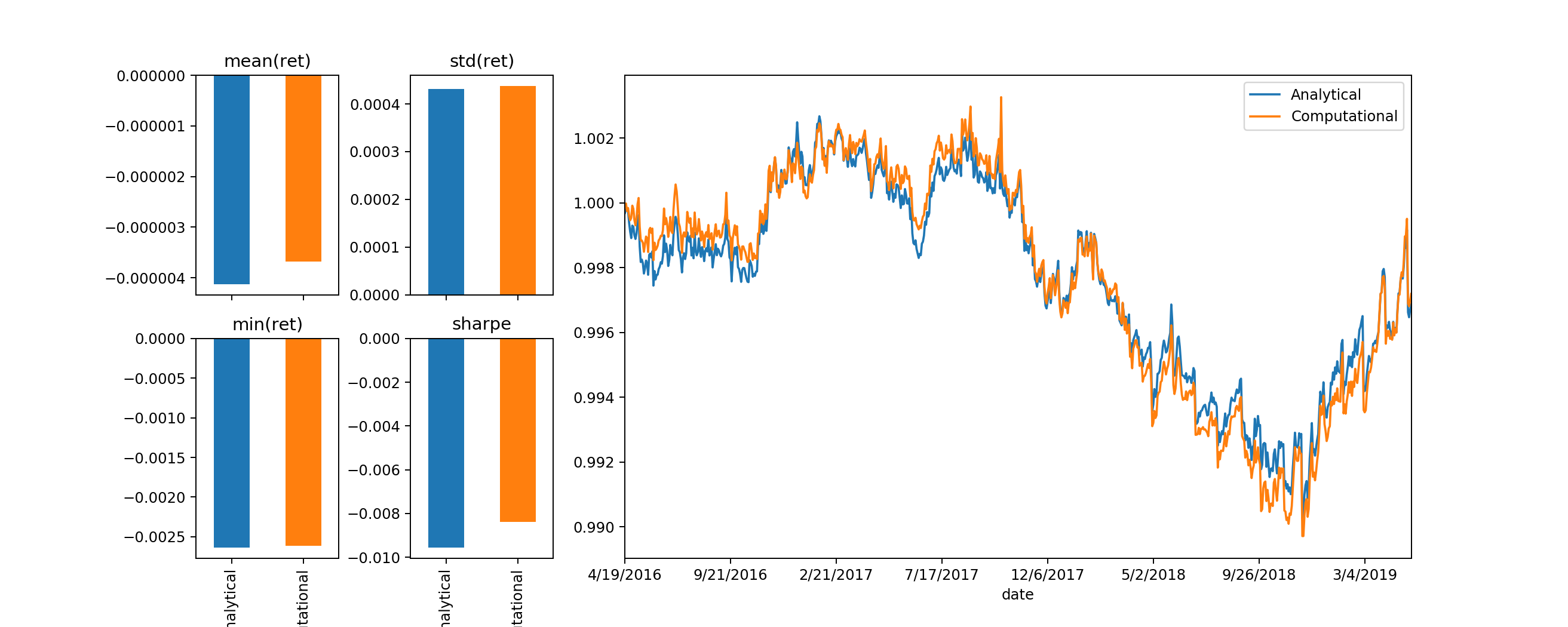
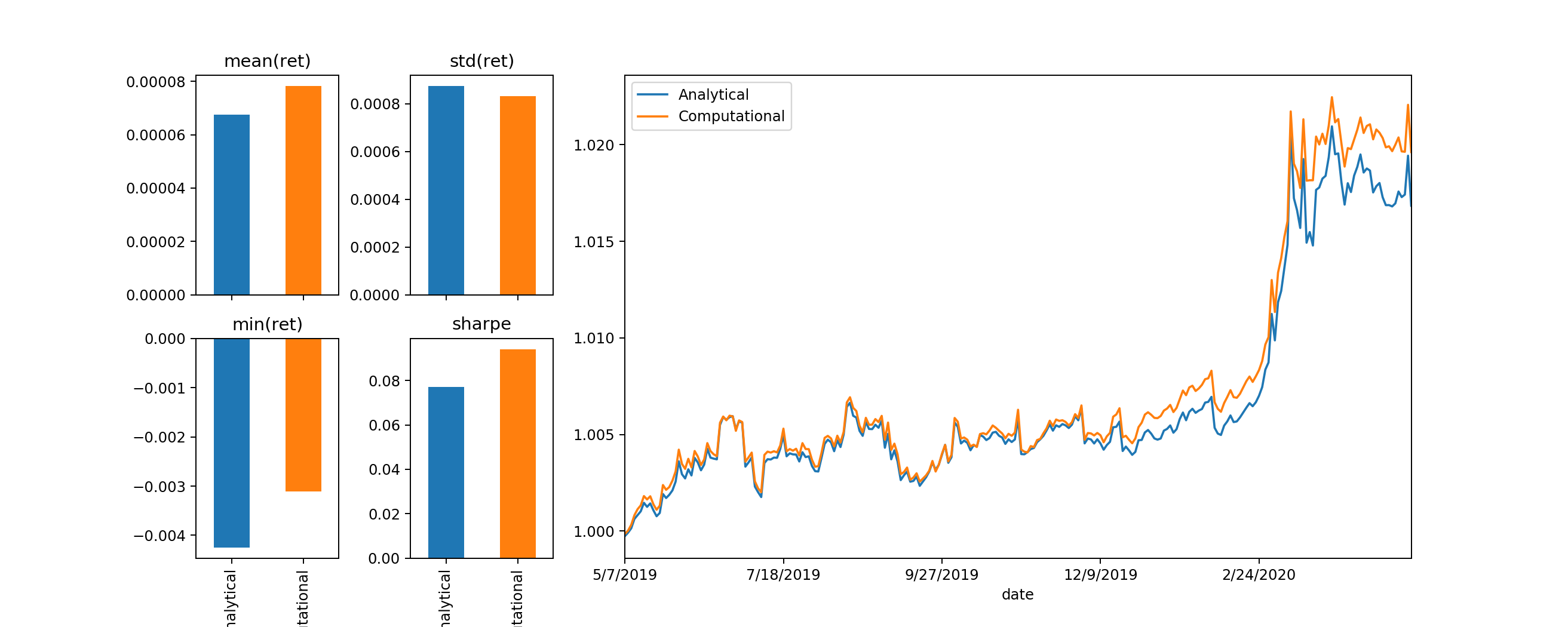
Conclusions & Remarks
- The discrepancies between our analytical & computational approaches are very small. I theorize that this is due to either when approximating the inverse covariance matrix when solving analytically, or computational errors. I will add an explanation once I have empirically identified the problem.
- It is much faster to use the analytical method to compute our Minimum Variance Portfolio, especially as M increases to which requires more combinations for iterations when utilizing computational approach.
- We tend to opt for computation when we don’t have the concrete mathematics to solve for the optimization problem, specifically when the constraint is not an equality constraint (=) but rather inequality constraints (<,>,<=,>=)
- The mathematics can get laborious the more we complexify our Lagrangian, so I will add them more if we have the time. For now, for demonstrative purposes it’s much easier to use the computational approach for adding more constraints or changing optimization target*
For example, instead of \(\sigma_p\), maybe we can change it to \(\boldsymbol{I_p}\), and perform maximization instead of minimization. Note that this is NOT the tangency portfolio, as tangency portfolio is about mean-variance optimization, a linear/quadratic system that can be analytically solved, optimizing directly to the quotient ratio can only be performed computationally. Perhaps I will demonstrate this as well later, although it is fairly easy to change up the code (check out Scipy Optimization Documentation)
2. Eigen Portfolios
Recall our brief introduction in the first post, eigen portfolios are simply the eigen vectors “scaled” by the summation of its components. We need to address the following important fundamental concepts & empirical findings:
-
The idea of an eigen portfolio is simply an allocation vector that aligns itself in the exact direction of the eigen vector.
-
For the eigen vectors \(e_{i} = \begin{vmatrix} e_{i_1}\\ e_{i_2}\\ \vdots\\ e_{i_M} \end{vmatrix}\), each being a unit vector such that \(\left \| e_i \right \| = 1\), when multiplied (scaled) by the summation of its components, we obtain the eigen portfolios \(w_{e_i} = \frac{e_i}{e_i \cdot \vec{\boldsymbol{1}}} = \frac{e_i}{\sum_{n=1}^{M}e_{i_n}}\)
-
The eigen portfolios \(w_{e_i}\) no longer are unit vectors, meaning that \(\left \| w_{e_i} \right \| \neq 1\).
-
The eigen values \(\lambda_i\) are interpreted as an exposure factor associated with its respective eigen portfolio \(w_{e_i}\).
-
It is empirically proven, through other research works, that \(w_{e_1}\), being the eigen portfolio associated with the eigen vector with the largest eigen value, is the market portfolio, given the universe of M securities comprising the market.
Modifying our function written to extract the eigen pairs in the previous post, below function scaled the eigen vectors with their weights summation into eigen portfolios and return the portfolios’ weights along with everything else, with some extra information on the eigen values (\(\lambda_i\)):
def EIGEN(_ret_):
    _pca = PCA().fit(_ret_)
    eVecs = _pca.components_
    eVals = _pca.explained_variance_
    _eigenNames = ["eigen_"+str(e+1) for e in range(len(eVals))]
    _eigenValues = pd.Series(eVals,index=_eigenNames,name="eigenValues")
    _eigenVectors = pd.DataFrame(eVecs.T,index=_ret_.columns,columns=_eigenNames)
    _eigenPortfolios = pd.DataFrame({e:(_eigenVectors[e]/_eigenVectors[e].sum()) for e in _eigenVectors})
    return {"vectors":_eigenVectors,"portfolios":_eigenPortfolios,
            "lambdas":pd.DataFrame({
                    "values":_eigenValues,
                    "explained_ratio":pd.Series(data=_pca.explained_variance_ratio_, index=_eigenPortfolios.columns),
                    "explained_cum_ratio":pd.Series(data=_pca.explained_variance_ratio_.cumsum(),
                                                    index=_eigenPortfolios.columns)})}
Recall that we are working with the sector Others, containing 35 securities representing a diverse pool of different funds & indexes, comprising the entire “market” as much as we can, with components as independent they can, ranging from different asset classes (stocks, commodities, T-bills, etc) as well as domestic & foreign securities (refer to the table above in our Preparation section for information).
Throughout our work, we will repeatedly construct an allWeights table of different allocations weights for bulk evaluations. Given an allocation weight of M securities being an M-dimensional vector, we write a simple function calculating the vectors’ norms and absolute sizes:
def weights_info(all_w):
    return pd.DataFrame({
            "norm":pd.Series(data=[np.linalg.norm(all_w[w]) for w in all_w.columns],index=all_w.columns),
            "absolute_size":pd.Series(data=[abs(all_w[w]).sum() for w in all_w.columns],index=all_w.columns)})
First, we will obtain the eigen portfolios along with other informations computed from our EIGEN() function written above, calculated from in-sample data:
_eigen_ = EIGEN(RET)
Checking the information of the first 10 eigen values \(\lambda_i\):
_eigen_["lambdas"].head(10)
| values | explained_ratio | explained_cum_ratio | |
|---|---|---|---|
| eigen_1 | 0.002100 | 0.491341 | 0.491341 |
| eigen_2 | 0.000566 | 0.132433 | 0.623774 |
| eigen_3 | 0.000318 | 0.074486 | 0.698259 |
| eigen_4 | 0.000272 | 0.063558 | 0.761817 |
| eigen_5 | 0.000182 | 0.042652 | 0.804469 |
| eigen_6 | 0.000145 | 0.033929 | 0.838398 |
| eigen_7 | 0.000100 | 0.023477 | 0.861875 |
| eigen_8 | 0.000095 | 0.022277 | 0.884151 |
| eigen_9 | 0.000084 | 0.019615 | 0.903766 |
| eigen_10 | 0.000061 | 0.014161 | 0.917926 |
Observe cummulatively, the first 10 eigen vectors “explain” ~90% of the total variance of 35 securities, where ~50% of total variance can be explained by the first eigen vector. We interpret this as that if we align ourselves, as a portfolio, being an eigen portfolio, with such vector, we are exposing ourselves to “most volatility” in such direction. With that logic, the following the direction of the last eigen vector would put us at the “least volatility.” Keep in mind we are talking about eigen vectors, not portfolios, that explain the total variance, as we will observe that is not always being the case for all portfolios entailed.
First, we will take a look at eigen portfolios and compute their weights information:
eigenWeights = _eigen_["portfolios"]
eigenWeights_info = weights_info(eigenWeights)
Observe the interesting result on how long the eigen portfolio allocation vectors are, with some being extremely “leveraged,” if anything unrealistic. This is actually related with the content of Random Matrix Theory presented further below.
eigenWeights_info
| norm | absolute_size | |
|---|---|---|
| eigen_1 | 0.197186 | 1.027671 |
| eigen_2 | 1.033669 | 3.356501 |
| eigen_3 | 1.108126 | 4.042055 |
| eigen_4 | 0.738428 | 3.201952 |
| eigen_5 | 0.961829 | 4.364877 |
| eigen_6 | 5.231791 | 22.957460 |
| eigen_7 | 1.972259 | 7.809851 |
| eigen_8 | 50.131156 | 205.898791 |
| eigen_9 | 3.205860 | 10.626309 |
| eigen_10 | 11.320662 | 42.868276 |
| eigen_11 | 10.567652 | 51.284834 |
| eigen_12 | 2.354090 | 8.967522 |
| eigen_13 | 4.622340 | 19.529794 |
| eigen_14 | 0.899101 | 3.563544 |
| eigen_15 | 6.078077 | 22.636898 |
| eigen_16 | 1.434698 | 6.106855 |
| eigen_17 | 23.261350 | 98.144726 |
| eigen_18 | 6.366735 | 21.457009 |
| eigen_19 | 4.981591 | 19.724526 |
| eigen_20 | 2.246686 | 9.007742 |
| eigen_21 | 2.860722 | 9.523268 |
| eigen_22 | 5.484353 | 19.521107 |
| eigen_23 | 33.792455 | 143.153880 |
| eigen_24 | 1.648818 | 6.553200 |
| eigen_25 | 4.091599 | 12.865818 |
| eigen_26 | 2.318411 | 8.688983 |
| eigen_27 | 4.305217 | 11.602049 |
| eigen_28 | 4.542940 | 14.122884 |
| eigen_29 | 106.344035 | 301.257355 |
| eigen_30 | 58.863324 | 169.725907 |
| eigen_31 | 28.727893 | 94.880161 |
| eigen_32 | 38.456731 | 118.547899 |
| eigen_33 | 1.272343 | 2.699258 |
| eigen_34 | 7.439441 | 17.137791 |
| eigen_35 | 1.481638 | 2.210459 |
Looking at eigen_1, given all weights must already satisfied the components summation of 1, the absolute summation is also the closest to 1. If we plot out the weights for eigen_1, we obtain:
eigenWeights["eigen_1"].sort_values().plot.bar(title="First Eigen Portfolio Weights")
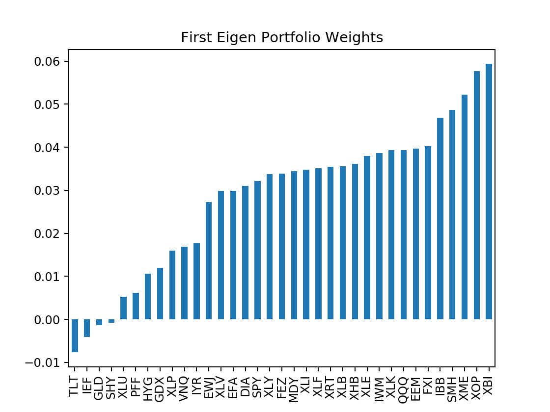
Notice how the eigen_1 weights have the majority of positive allocations in various large market indexes, specifically U.S. equities market. This support our statement above on it being the market portfolio. Notice how 3/4 of our negative allocations, or short positions, are in Treasury Bills (IEF, SHY, TLT), all statistically exhibit negative correlation with the market. The last short resides in GLD , being specifically gold, not are just significantly smaller than the rest but also hedged out in weights with another gold index GDX.
Meanwhile, if we plot the eigen_2 portfolio weights, we have:
eigenWeights["eigen_2"].sort_values().plot.bar(title="Second Eigen Portfolio Weights")
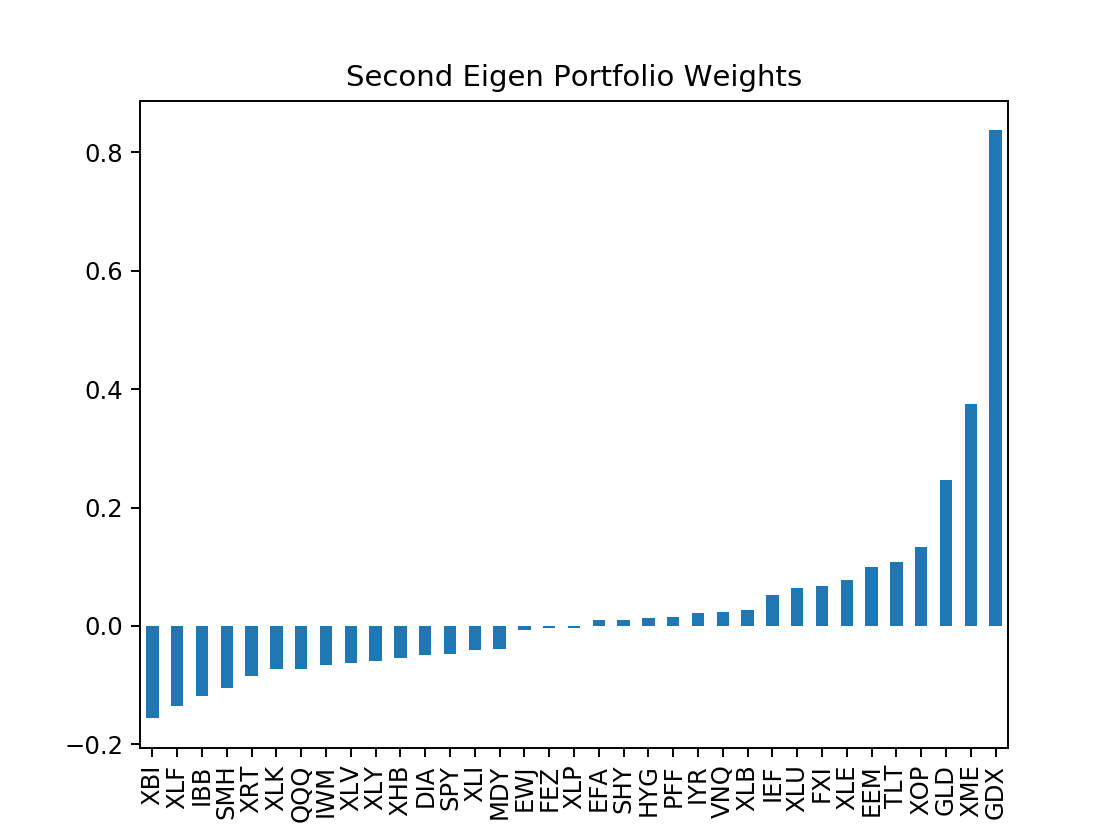
The largest positive weights are now allocated towards ones that are negative & smaller in the first eigen portfolio, that being Treasury & Gold. In addition, subsequent majority of the weights go towards indexes of commodities & energy (XME,XLE,XOP,etc..) as well as foreign securities (EWJ, FXI)
Now that we have extracted the eigen portfolios weights from in-sample data as eigenWeights, moving forward, we will construct an allWeights table, adding the Minimum Variance Portfolio into in addition with the eigenWeights, then proceed on recalculating the weights information:
allWeights = pd.concat([eigenWeights,minVar(RET.cov()).reindex(eigenWeights.index)],1)
allWeights_info = weights_info(allWeights)
Proceed on performing evaluations of allWeights on BOTH in-sample & out-sample:
inSample_evals = evaluate_bulk_w(RET,allWeights)
outSample_evals = evaluate_bulk_w(RET_outSample,allWeights)
Plotting results for the performance evaluations of the First 5 Eigen Portfolios, we obtain:
to_plot = ["eigen_1","eigen_2","eigen_3","eigen_4","eigen_5"]
plot_bulk_evals(inSample_evals,to_plot=to_plot,plot_title="In-Sample")
plot_bulk_evals(outSample_evals,to_plot=to_plot,plot_title="Out-Sample")
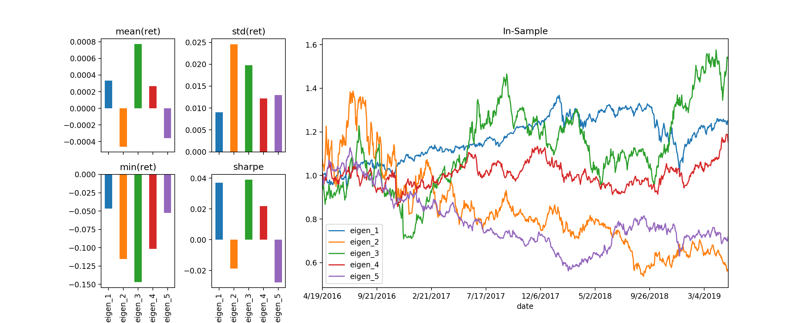

The interesting thing to point out is the out-sample result, the timeframe to which when the latest COVID-19 market crash occured eigen_3 portfolios exhibit positive performance in comparison to the rest (as well as in-sample). Looking at the weights of such portfolio, we observe:
allWeights["eigen_3"].sort_values().plot.bar(title="Third Eigen Portfolio Weights")
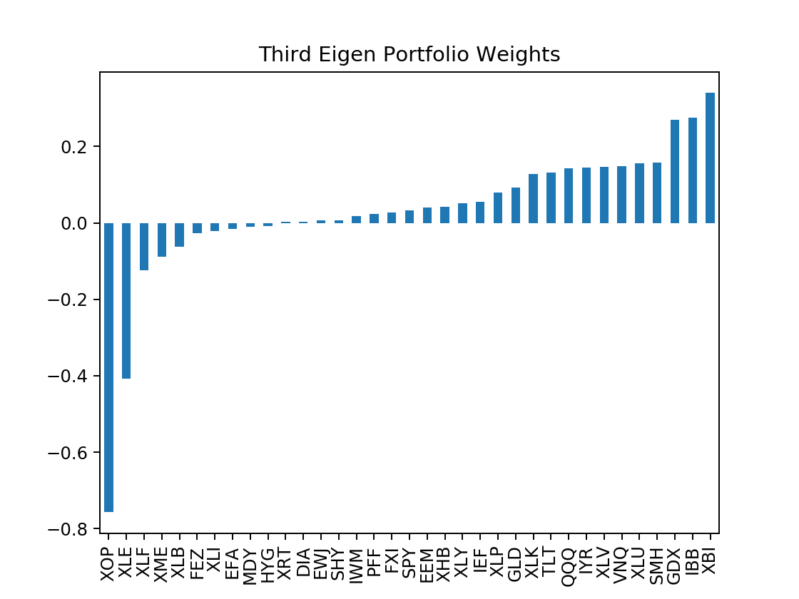
This portfolio shorts the majority of SPDR sector indexes and hedges out with other indexes that mirrored the same thing, yet longing the majority of Treasury Bills & Gold indexes, to which explains its relatively superior performance for the COVID-19 market crash, while yet retaining its decent performance when market was bullish.
Observe the correlational heatmap for the returns of portfolios in allWeights, again extracted from in-sample data, on in-sample and out-sample data:
f = plt.figure()
inSample_ax = f.add_subplot(121,title="In-Sample")
inSample_ax.imshow(inSample_evals["returns"].corr())
outSample_ax = f.add_subplot(122,title="Out-Sample")
a = outSample_ax.imshow(outSample_evals["returns"].corr())
cbar = f.colorbar(a, ticks=[-1, 0, 1])
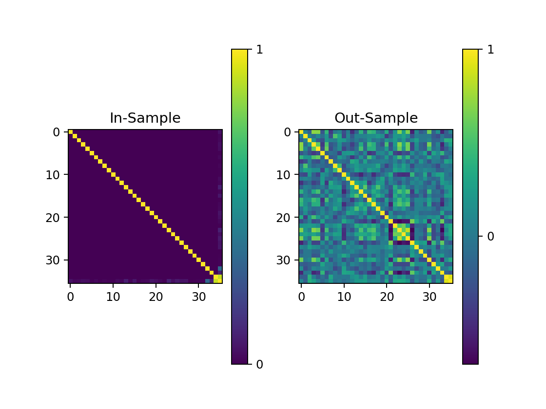
Notice how the eigen portfolios exhibit 0 correlation to each other on in-sample data, yet moving to out-sample, such effect is diminished. Meanwhile, at the bottom-right corner of the heatmap represents the Minimum Variance Portfolio, somehow exhibiting consistent correlation with the last eigen portfolios
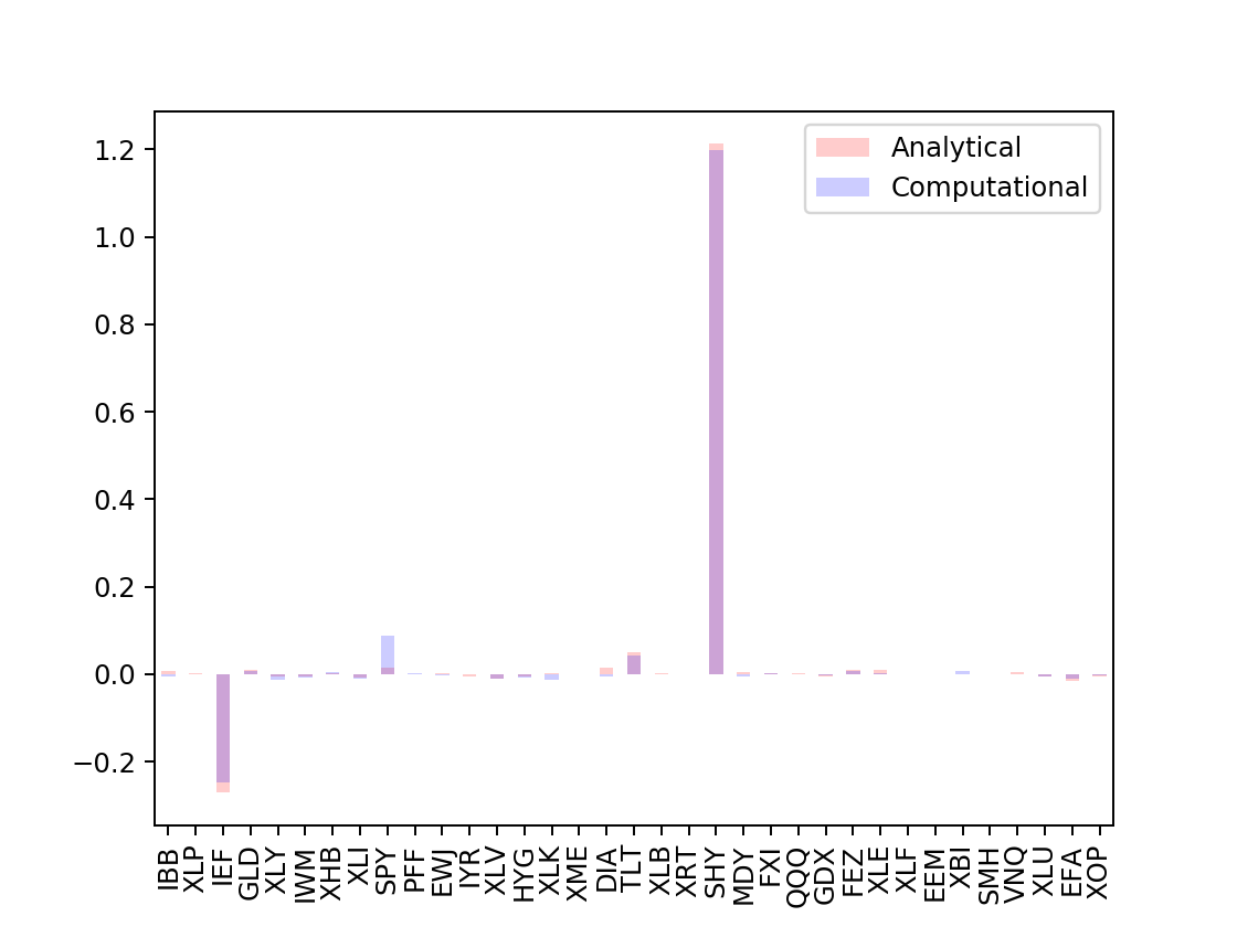
Now, if we take a look at the evaluations of the Minimum Variance Portfolio with the LAST eigen portfolio (eigen_35), associating with the smallest eigen value:
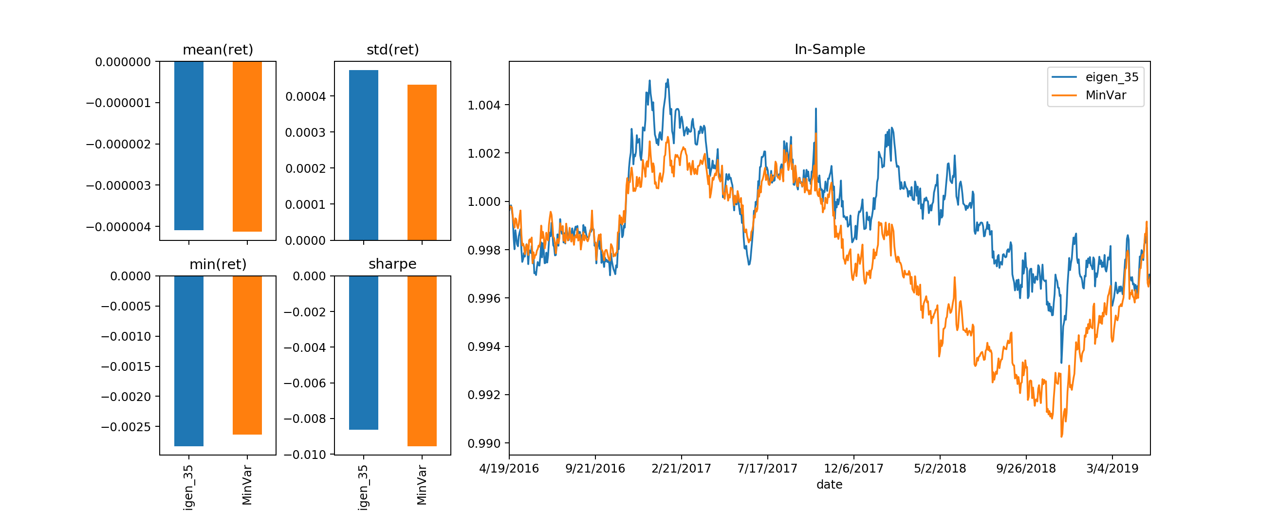
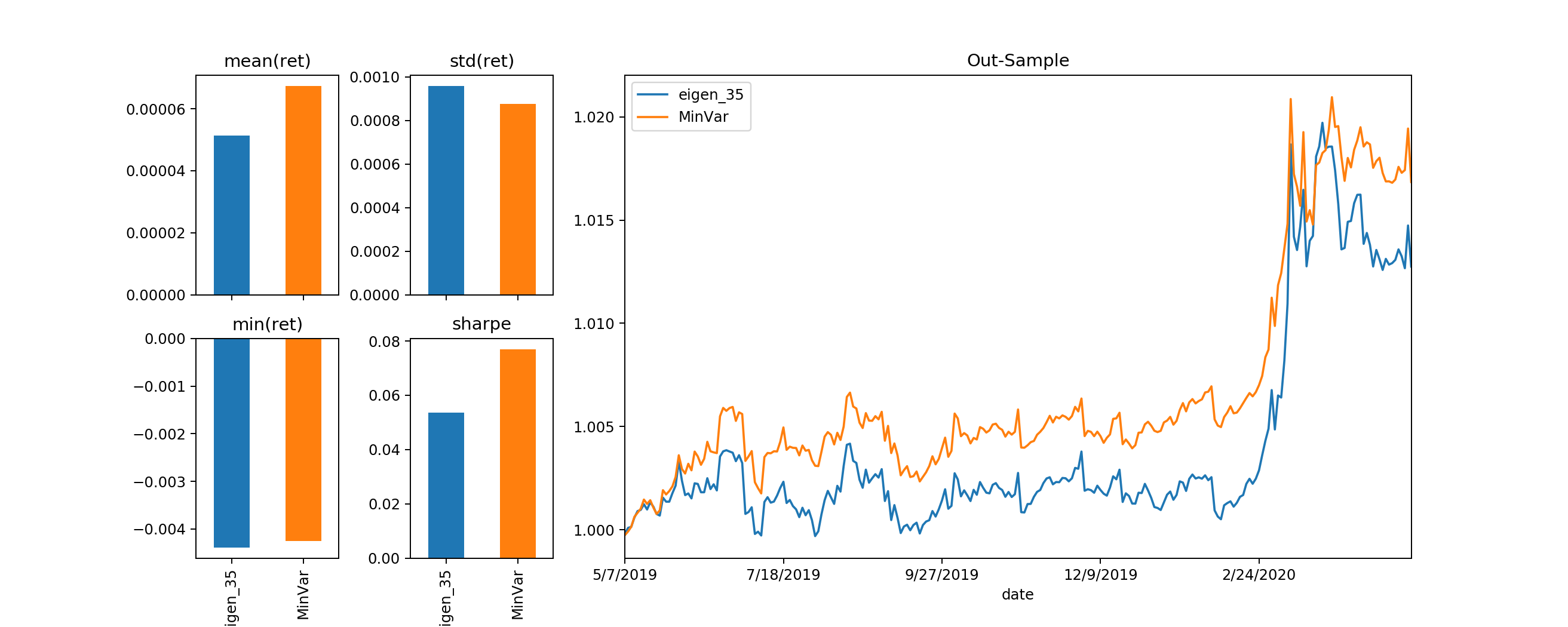
They are very closely “related” with each other, though the Minimum Variance Portfolio still beating the eigen_35 portfolio. Observe the weights bar plot, as well as the dot product between the two allocation vector, as well as their angle from each other, represents at \(cos(\theta)\) (1 means they line up exactly with each other):
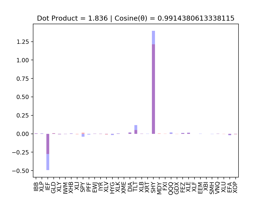
They are aligned very close with each other, with one allocation vector just basically has a higher norm than the other. This further supports our initial hypothesis on the “meaning” of eigen portfolios & eigen values.
Random Matrix Theory
The advanced mathematical technique to be presented belongs to a larger topic umbrella called Random Matrix Theory, specifically inspired by Alan Edelman’s lecture notes for a class on such topic at MIT. There are much more to be learned & explore as per for myself as well, although what will be presented are implementations & testings, performed personally, that have yielded positive empirical results.
The main concept we are addressing is directly related with portfolio optimization. Shortly put, a significant arena within Random Matrix Theory (RMT) is understanding the distribution of eigen values in any large random matrix. What we are specifically working on is a square matrix referred to as the Wilshart Matrix, having such distribution stemmed from fact of Gaussian orthogonal ensemble (or GOE) having its distribution being invariant under any orthogonal transformations, aka eigen decompositions we performed thus far.
The bomb-shell of an application to our current objective lies under the belief that:
Under certain conditions, there exists a theoretical range of eigen values, followed by such distribution, such that the ones outside of such theoretical range are values that contain actual useful information, where the rest inside are random noises of interactions within the data.
Correlation \(\boldsymbol{C_{\rho}}\) & Covariance \(\boldsymbol{C_{\sigma}}\)
As we have observed so far, Portfolio Optimization always involves the Covariance Matrix \(\boldsymbol{C_{\sigma}}\) being an M x M Hermitian Matrix that directly computed from any input N x M returns matrix \(RET\), containing N data points of M securities.
It is important to note that the entries of \(\boldsymbol{C_{\sigma}}\) are not bounded. However, aside from PCA, \(\boldsymbol{C_{\sigma}}\) can also be decomposed into a multiplication of other important matrices, specifically being the Standard Deviation Matrix \(\boldsymbol{D}^{1/2}\) and the Correlation Matrix \(\boldsymbol{C_{\rho}}\)
\(\boldsymbol{D}^{1/2}\) is an M x M diagonal symmetric matrix, where for \(i,j = 1,2,...,M\) of M securities, each diagonal entry \(d_{ii} = \sigma_{i}\) represents the standard deviation of security i, while the other entries where \(i \neq j\), \(d_{ij} = 0\), such that:
\[\boldsymbol{D}^{1/2} = \begin{vmatrix} \sigma_{1} &0 &\cdots &0 \\ 0 &\sigma_{2} &\cdots &0 \\ \vdots &\vdots &\ddots &\vdots \\ 0 &0 &\cdots &\sigma_{M} \end{vmatrix}\]\(\boldsymbol{C_{\rho}}\) is also an M x M symmetric matrix, where each entry represents the correlation value between two securities. For \(i,j = 1,2,...,M\), where \(i \neq j\), \(c_{ij} = \rho_{ij} = \frac{\sigma_{ij}}{\sigma_{i} \sigma_{j}}\), thus by such definition, the diagonal entries \(c_{ii} = 1\), as the correlation of a security to itself is 1, such that:
\[\boldsymbol{C_{\rho}} = \begin{vmatrix} 1 &\rho_{12} &\cdots &\rho_{1M} \\ \rho_{21} &1 &\cdots &\rho_{2M} \\ \vdots &\vdots &\ddots &\vdots \\ \rho_{M1} &\rho_{M2} &\cdots &1 \end{vmatrix}\]Putting it together, we have our Covariance Matrix decomposed as:
\[\boldsymbol{C_{\sigma}} = \boldsymbol{D}^{1/2} \cdot \boldsymbol{C_{\rho}} \cdot \boldsymbol{D}^{1/2}\]Similar to what we did before, performing PCA on \(RET\), basically Eigen Decomposition on \(\boldsymbol{C_{\sigma}}\), this time, we instead proceed on applying Eigen Decomposition on \(\boldsymbol{C_{\rho}}\).The result exhibit these important fundamentals:
- The eigen vectors \(e_i\) obtained from \(\boldsymbol{C_{\rho}}\) is the same as \(\boldsymbol{C_{\sigma}}\)
- For \(M\) securities, constructing the symmetric M x M Correlation Matrix, their eigen values will follow \(\sum_{i=1}^{M}\lambda_i = M\)
Wilshart & Correlation Matrix \(\boldsymbol{C_{\rho}}\)
Given any N x M matrix \(X\), with its entry values being real & distributed in \(x_{ij} \sim \mathcal{N}(0,\sigma^2)\), resulting in its conjugate being the tranpose, \(X^* = X^\top\), we have: \(W = X^* \cdot X = X^\top \cdot X\)
\(W\) here, being a symmetric matrix is called a Wilshart Matrix.
Now, if we normalize the returns matrix \(RET\) into \(\bar{RET}\) such that:
\[\bar{RET} = \begin{vmatrix} \vec{\bar{r_1}} & \vec{\bar{r_2}} & \cdots &\vec{\bar{r_M}} \end{vmatrix}\]where \(\vec{\bar{r_i}} = \begin{vmatrix} \bar{r_{i_1}}\\ \bar{r_{i_2}}\\ \vdots\\ \bar{r_{i_N}} \end{vmatrix}\) being the N returns of security i normalized by standard deviation so that \(\sigma_{\bar{r_i}} = 1\), then:
\(\boldsymbol{C_{\rho}} = \bar{RET}^T \cdot \bar{RET}\) Just like the Wilshart Matrix, with \(W=\boldsymbol{C_{\rho}}\) and \(X = \bar{RET}\)
We know that the Correlation Matrix \(\boldsymbol{C_{\rho}}\), viewed as a “normalized version” of the Covariance Matrix \(\boldsymbol{C_{\sigma}}\), being bounded between (-1,1) with entries being real values:
\[\boldsymbol{C_{\rho}} = \begin{vmatrix} 1 &\rho_{12} &\cdots &\rho_{1M} \\ \rho_{21} &1 &\cdots &\rho_{2M} \\ \vdots &\vdots &\ddots &\vdots \\ \rho_{M1} &\rho_{M2} &\cdots &1 \end{vmatrix}\]has its diagonal entries always being 1, can somewhat perceived to be a Wilshart Matrix under the assumption that the True \(\boldsymbol{C_{\rho}}\) is the Identity Matrix
\[\boldsymbol{I} = \begin{vmatrix} 1 &0 &\cdots &0 \\ 0 &1 &\cdots &0 \\ \vdots &\vdots &\ddots &\vdots \\ 0 &0 &\cdots &1 \end{vmatrix}\]Equivalent to the definition of the entries of a Wilshart Matrix entries distributed in \(x_{ij} \sim \mathcal{N}(0,\sigma^2)\), to which in the context of our Correlation Matrix \(\boldsymbol{C_{\rho}}\), we take \(\sigma^2 = 1\) without loss of generality.
Wigner’s Semi-Circle
In short, according to the Wigner’s semi-circle Law, for an M x M square matrix \(\boldsymbol{\bar{A}}\) with its entries distributed as \(\bar{a}_{ij} \sim \mathcal{N}(0,\sigma^2)\), we define:
\[\boldsymbol{A}_{M} = \frac{1}{\sqrt{2M}}(\boldsymbol{\bar{A}} + \boldsymbol{\bar{A}}^\top )\]\(\boldsymbol{A}_{M}\) is now a symmetric matrix with entries \(a_{ij}\) distributed with their variances \(\sigma_{a_{ij}}^2\) as:
\[\sigma_{a_{ij}}^2 = \left\{\begin{matrix} \frac{\sigma^2}{M} \; \; \;if \; \; i \neq j\\ \\ \frac{2\sigma^2}{M} \; \; \;if \; \; i = j \end{matrix}\right.\]Wigner’s semi-circle state that, as \(M \rightarrow \infty\), the density of eigen values of \(\boldsymbol{A}_{M}\) is given as:
\[\rho(\lambda) := \left\{\begin{matrix} \frac{1}{2\pi \sigma^2} \sqrt{4\sigma^2 - \lambda^2}\; \; \; if\; \; \;\left | \lambda \right | \leq 2\sigma\\ \\ 0 \; \; \; if\; \; \;\ otherwise. \end{matrix}\right.\]This finding of modeling the distribution of a random square matrix under some Gaussian Distribution resulting in the universal constant \(\pi\), connected with the idea of Gaussian Orthogonal Ensemble mentioned above leads to the next important theorem that we will apply to Portfolio Optimization
Marchenko-Pastur Theorem
There exists a probability density function (PDF) called the Marchenko-Pastur Distribution, stating that:
For a symmetric MxM Wilshart Matrix \(W\), constructed from any random N x M matrix \(X\) with entries distributed in \(\mathcal{N}(0,\sigma^2)\), such that \(W = X^* \cdot X = X^\top \cdot X\), As the limit \(N,M \rightarrow \infty\), with the ratio \(Q = \frac{N}{M} \geq 1\), the density of eigen values of \(W\) is given as:
\[\rho (\lambda) = \frac{Q}{2\pi \sigma^2}\frac{\sqrt{(\lambda_{+} - \lambda)(\lambda - \lambda_{-})}}{\lambda}\]Where \(\lambda_{+}\) and \(\lambda_{-}\) are the maximum and minimum eigen values respectively, given as:
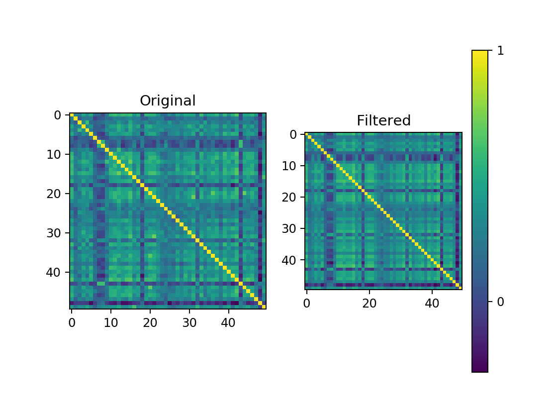
\[\lambda_{\pm} = \sigma^2(1 \pm \sqrt{\frac{1}{Q}})^2\]Values that lie inside of the theoretical range are perceived to be noises of data interactions thus we can filter of them out, keeping ones that remain outside of such range as eigen values that hold actual information, to which in our case being the true correlational information.
def _RMT_(RET,Q=None,sigma=None,include_plots=False,
                          exclude_plotting_outliers=True,auto_scale=True):
    #----| Part 1: Marchenko-Pastur Theoretical eVals
    T,N = RET.shape
    Q = Q or (T/N) #---| optimizable
    sigma = sigma or 1 #---| optimizable
    min_theoretical_eval = np.power(sigma*(1 - np.sqrt(1/Q)),2)
    max_theoretical_eval = np.power(sigma*(1 + np.sqrt(1/Q)),2)
    theoretical_eval_linspace = np.linspace(min_theoretical_eval,max_theoretical_eval,500)
    def marchenko_pastur_pdf(x,sigma,Q):
        y=1/Q
        b=np.power(sigma*(1 + np.sqrt(1/Q)),2) # Largest eigenvalue
        a=np.power(sigma*(1 - np.sqrt(1/Q)),2) # Smallest eigenvalue
        return (1/(2*np.pi*sigma*sigma*x*y))*np.sqrt((b-x)*(x-a))*(0 if (x > b or x <a ) else 1)
    pdf = np.vectorize(lambda x:marchenko_pastur_pdf(x,sigma,Q))
    eVal_density = pdf(theoretical_eval_linspace)

    #-----| Part 2a: Calculate Actual eVals from Correlation Matrix & Construct Filtered eVals
    corr = RET.corr()
    eVals,eVecs = np.linalg.eigh(corr.values)
    noise_eVals = eVals[eVals <= max_theoretical_eval]
    outlier_eVals = eVals[eVals > max_theoretical_eval]
    filtered_eVals = eVals.copy()
    filtered_eVals[filtered_eVals <= max_theoretical_eval] = 0
    #-----| Part 2b: Construct Filtered Correlation Matrix from Filtered eVals
    filtered_corr = np.dot(eVecs,np.dot(
                        np.diag(filtered_eVals),np.transpose(eVecs)
                                        ))
    np.fill_diagonal(filtered_corr,1)
    #----| Part 2c: Construct Filtered Covariance Matrix from Filtered Correlation Matrix
    cov = RET.cov()
    standard_deviations = np.sqrt(np.diag(cov.values))
    filtered_cov = (np.dot(np.diag(standard_deviations),
                        np.dot(filtered_corr,np.diag(standard_deviations))))
    result = {
        "raw_cov":cov,"raw_corr":corr,
        "filtered_cov":pd.DataFrame(data=filtered_cov,index=cov.index,columns=cov.columns),
        "filtered_corr":pd.DataFrame(data=filtered_corr,index=corr.index,columns=corr.columns),
        "Q":Q,"sigma":sigma,
        "min_theoretical_eval":min_theoretical_eval,
        "max_theoretical_eval":max_theoretical_eval,
        "noise_eVals":noise_eVals,
        "outlier_eVals":outlier_eVals,
        "eVals":eVals,"eVecs":eVecs
    }
    if include_plots:
        #----| Plot A = Eigen Densities Comparison of Actual vs Theoretical
        MP_ax = plt.figure().add_subplot(111)
        eVals_toPlot = eVals.copy() if (not exclude_plotting_outliers) else eVals[eVals <= max_theoretical_eval+1]
        MP_ax.hist(eVals_toPlot, density = True, bins=100)
        MP_ax.set_autoscale_on(True)
        MP_ax.plot(theoretical_eval_linspace,eVal_density, linewidth=2, color = 'r')
        MP_ax.set_title(("Q = "+ str(Q) + " | sigma = " + str(sigma)))
        result["MP_ax"] = MP_ax

        #----| Plot B = Original vs Filtered Correlation Matrix (from filtered eVals)
        f = plt.figure()
        FILTERED_ax = f.add_subplot(121,title="Original")
        FILTERED_ax.imshow(corr)
        FILTERED_ax = f.add_subplot(122,title="Filtered")
        a = FILTERED_ax.imshow(filtered_corr)
        cbar = f.colorbar(a, ticks=[-1, 0, 1])
        result["FILTERED_ax"] = FILTERED_ax
    return result
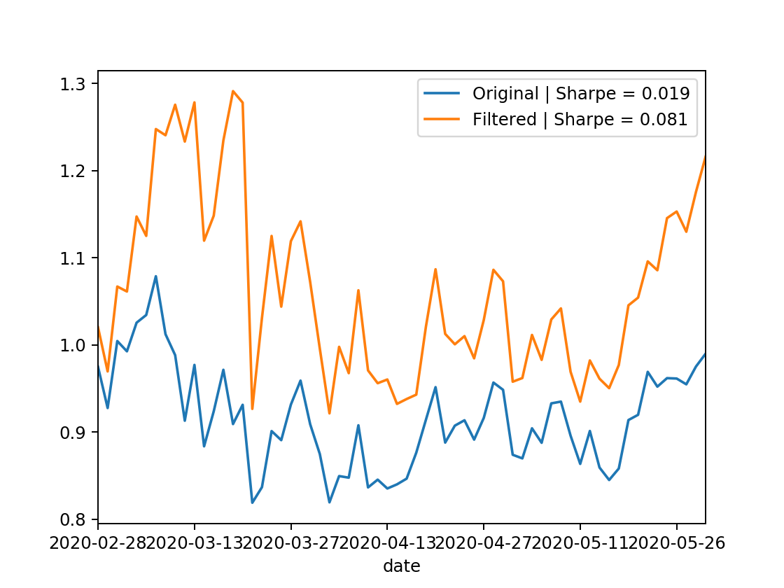
 In-Sample
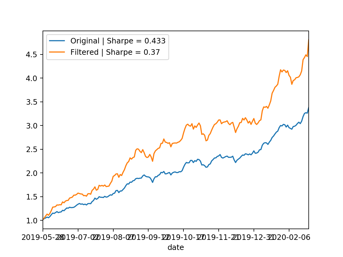 Out-Sample