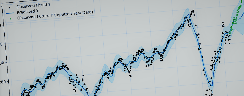
Time-Series Forecasting: FBProphet & Going Bayesian with Generalized Linear Models (GLM)

In the recent years, Facebook released an open-source tool for Python & R, called fbprophet, allowing scientists & developers to not just tackle the complexity & non-linearity in time-series analysis, but also allow for a robust regression model-building process, to forecast any time-series data while accounting for uncertainty in every defined variables (priors & posteriors) of any built models.

After spending some time reading Facebook’s published research paper on fbprophet, conducted by their mathematicians, as well as breaking down the developers’ codes from their open-source repository (Python), I was able to understand, in details, the mathematics & computational executions, thus built my own time-series forecaster with additional complexities added, utilizing their mathematical foundations.

As an attempt of mine to explain the model in more applicable details, and alternatively recreate it with further implementations added, in this post, we will explore:

The difference between Ordinary v.s. Generalized Linear Models (GLM) & why we are using GLM to build time-series forecasters.
The benefits of “going Bayesian”
The mathematics and backend code of FBProphet.

Such that, at the end, we aim to build our own version in Python with additional flexibility & creative concepts added, utilizing PyMC3 instead of Stan (like fbprophet does) as backend sampler.

In addition, I will not spend much time talking about PyMC3, as you can navigate here to explore. It’s an amazing sampler for probabilistic models built in Python, that implements frontier computational algorithms for regressions of various distributions in our built models. In addition with a rich library of variational inferencing methods, it also use them to accelerate MCMC simulations for sampling/fitting purposes.

1. The Superiority of Generalized Linear Models

Linearity is the foundational language that explains the totality of composition for any reality we are trying to model, as regression becomes the basis for the overarching factor-modeling technique in the modern data-driven world, especially neural network models in Machine Learning.

However, the main difference between a regular ordinary linear regression model and a generalized one falls under the concept of symmetry & normality, a theoretical zero-sum framework towards reality as a whole (not as what we observed incrementally through time).

The intuition, as I summarize below, is best explained by this Wikipedia page:

Ordinary linear regression predicts Y, the expected value of a given unknown quantity (the response variable, a random variable), as a linear combination of a set of observed values X’s (predictors):

\[Y = \sum \alpha_{i} X_{i}\]

This is appropriate when the response variable can vary indefinitely in either direction.
When asked about the distribution of such predicted values, we only need \(\mu\) and \(\sigma\) to describe the symmetric property of its deviation.

However this is not generally true when tackling problems from real-world data, as such data typically are not normally distributed, as many exhibit certain properties aside from just skewness & kurtosis, but rather fatter tails or positively bounded, etc. For example (by Wiki):

Suppose a linear prediction model learns from some data (perhaps primarily drawn from large beaches) that a 10 degree temperature decrease would lead to 1,000 fewer people visiting the beach. This model is unlikely to generalize well over different sized beaches.

Generalized linear models cover all these situations by allowing for response variables that have arbitrary distributions (rather than simply normal distributions), and for an arbitrary function of the response variable (the link function) to vary linearly with the predicted values (rather than assuming that the response itself must vary linearly). For example (by Wiki):

The case above of predicted number of beach attendees would typically be modeled with a Poisson distribution and a log link, while the case of predicted probability of beach attendance would typically be modeled with a Bernoulli distribution (or binomial distribution, depending on exactly how the problem is phrased) and a log-odds (or logit) link function.

In short, a generalized linear model covers all possible ways of how different distributions of difference factors, abstract or real, can “hierarchically” impact the defined distribution of the observed. This allows us to tackle complex time-series problems, especially ones that exhibit non-linearity, while retain uncertainty in our models, as well as not having to worry about data stationarity that classical time-series models, such as ARIMA, heavily rely on

2. Going Bayesian

All Bayesian techniques & implementations in modern days, even in machine learning neural networks, are built from statistical foundation pioneered by Thomas Bayes himself, back in the late 1700s, called Bayes Theorem:

\[P(A \mid B) = \frac{P(A) P(B \mid A)}{P(B)}\]

This approach of modeling variables, both the priors & posteriors, as distributions was not been heavily explored & implemented back then due to high computational demands. However in the last century, the recent accelerating technological advancement in both hardware & software, alongside with continuously improved ML learning algorithms, has allowed Bayesians to find themselves a vital role for data modelling approaches in modern days, especially in building complex models, like neural network, or multi-dimensional hierarchical GLM like what we are doing.

Let’s start by recalling the brief explanation about GLM from above:

Generalized Linear Models allow for response variables that have arbitrary distributions, and for an arbitrary function of the response variable to vary linearly with the predicted values (rather than assuming that the response itself must vary linearly)

Shortly put in details, implementation of Bayesian Statistics on time-series GLM is powerful due to:

The ability for us to define priors (initial beliefs) as any distributions with probability functions, thus \(P(A), P(B),...\), whereas such priors \(A, B, ...\) are variables/features that can be as abstract or realistic as we want.
We can formulate functions (link functions), as \(f(A,B,...)\) with defined priors variables \(A,B,...\), as transformed variables, to define our posteriors, being the observables. Thus, modeled as either a factor in a model to predict a selected target, or even the targets themselves, the posteriors can also be defined as distributions.
We can then update our prior beliefs with the arrival of new observed data, using Bayes’ Theorem, specifically the concept of conditional probability \(P(Y \mid X)\) (where \(X\) being a conditioned variable, either as a prior or a function of a group of priors), and vice versa as \(P(X \mid Y)\)

We will demonstrate these implementations in this post. To summarize:

The observable is the unknown posterior, to which conditionally dependent on the defined priors beliefs, where such priors are updated to “fit” the observable when new observable data arrive throughout time (hence variable t).

3. The Mathematics of FBProphet’s Model

Disclosure: The content below is somewhat a detailed summary, or rather a concise alternative explanation, based on my personal understanding of fbprophet’s GLM from reading their publication & repositories to build one of my own from scratch. If you want to check out the original published paper, click here.

Given \(\boldsymbol{Y}\) as the observable to fit & predict (data of prediction target), I often express the overarching model as:

\[\boldsymbol{Y}(t) \sim [\boldsymbol{G}(t) \cdot(1 + \boldsymbol{S}_{m}(t)) + \boldsymbol{S}_{a}(t)] \pm \boldsymbol{\epsilon}_{t}\]

where:

\(\boldsymbol{G}\) = Trend/Growth
\(\boldsymbol{S}_{m}\) = Multiplicative Seasonal Components
\(\boldsymbol{S}_{a}\) = Additive Seasonal Components
\(\boldsymbol{\epsilon}\) = Unknown Errors (set as \(\sigma\) of the observed by fbprophet)

Numerically Scaling Timestamps \(\boldsymbol{t}\)

As we are obviously trying to build a predictive model on time-series data, which under our assumptions moving forward, being all real numbers, or, simply put, such data are numeric data, aka integers & real numbers(floats). As time is basically the essence of our model-building, before we touch base on any components of our model, we need to define a numeric transformation on a given array of timestamp instances (they are not numbers), that, the aftermath result from such transformation, sortedly retains the periodicity & frequency of the original sorted array of timestamps given.

There are many ways of approaching this while avoiding look-ahead bias. I notice some define it as the integers field, though I personally opt for the same method fbprophet employs, scaling it directly through min-max standardization, into a “Gaussian-like” bound:

Given such array \(D\) containing \(N\) amount of timestamp instances, such that for example:

\[D = \begin{bmatrix} 1-3-2018 & 1-4-2018 &\cdots & 1-3-2020 \end{bmatrix}\]

The numeric transformation can be algorithmically defined as a standardizing procedure, taking in our timestamps array \(D\) and returning the numeric array \(\boldsymbol{t}\) with values between (0,1):

\[\boldsymbol{t} = \begin{bmatrix} 0 &\cdots & 1 \end{bmatrix}\]

Such that:

When fitting, we perform standardization on such array \(D\), as \(D_{fit}\), being a Min-Max scaling procedure:

\[\boldsymbol{t} = \frac{D - min(D)}{max(D) - min(D)}\]
Notice how such process cancels out our units and left us with purely numeric values, while capturing information of the timeframe we are working with.

When predicting, we use the fitted \(min(D)\) & \(max(D)\) values, aka \(min(D_{fit})\) & \(max(D_{fit})\) above, to perform the exact same scaling procedure on any given array \(D\), to which in predictive context viewed as \(D_{pred}\). The resulted \(\boldsymbol{t}\) values that are out of bound (0,1) represents stamps before (<0) or after (>1) the timeframe of data we fitted (the priors of our model on).

Modeling Trend [\(\boldsymbol{G}(t)\)]

Without worrying about their meanings at the moment, we first define 3 essential priors for our trend model:

\[k \sim \mathcal{N}(0,\theta)\] \[m \sim \mathcal{N}(0,\theta)\] \[\delta \sim Laplace(0,\tau)\]

where \(\theta\) and \(\tau\) being the scales of the priors’ distributions (or simply \(\sigma_G\) measuring the deviation of such priors). This is viewed as hyper-parameters for tuning with cross-validation (employed by fbprophet) or any other custom tuning methods.

As default, set by fbprophet:

\[\theta = 5\] \[\tau = 0.05\]

The effect of priors’ scaling values will be demonstrated in our work later on, as well as an extended creative idea on defining scales as priors themselves, although for now, we stick with them being as default constants.

We now explore their relative meanings & dimensions in our trend model:

\(\boldsymbol{k}\) [1-Dimensional] = Growth Rate
\(\boldsymbol{m}\) [1-Dimensional] = Growth Offset (or the “intercept” value)
\(\boldsymbol{\delta}\) [N-Dimensional] = Growth Rate Changepoints Adjustments

Notice how while \(k\) and \(m\) are 1 dimensional, or simply as constants, \(\delta\) is an \(N\)-dimensional variable, where such integer \(N\) is also a hyper-parameter, though not as important as prior scales, for tuning.

Our \(\delta\) here is somewhat similar to the commonly known concept in mathematics called Dirac Delta in differential equations, used to tackle problems with piece-wise regressions & step-functions.

Before finalizing our trend model, we also need to define a couple last components, although these will NOT be as priors with distributions needed to be sampled for fit but rather most of which are transformed variables and link functions, being calculation results using the defined priors & hyper-parameters above:

\[\boldsymbol{s}, A,\gamma\]

For every given \(\boldsymbol{t}\) as the numeric timesteps of \(K\) dimensional length, meaning there being K amount of timestamps given to fit or predict,
\[\boldsymbol{t} =\begin{bmatrix} t_1 & t_2 &\cdots & t_k \end{bmatrix}\]
and \(\delta\) of \(N\) dimensional length, representing \(N\) amount of changepoints occurring at values in \(\boldsymbol{t}\), we subsequently compute those N changepoint values from \(\boldsymbol{t}\), defined as \(\boldsymbol{s}\), being N-dimensional as well, such that:

For \(i = 1,2,...N\), where \(s_i \in \boldsymbol{t}\) and \(N \leq K\), we define
\[\boldsymbol{s} =\begin{bmatrix} s_1 & s_2 &\cdots & s_n \end{bmatrix}\]
We then compute the \(K\) x \(N\) matrix \(A\), called the Determining Matrix, with boolean entries as binaries (1 = True, 0 = False):
\[A_t = \begin{bmatrix} t_{1} \geq s_1 & t_{1} \geq s_2 & \dots & t_{1} \geq s_n \\ t_{2} \geq s_1 & t_{2} \geq s_2 & \dots & t_{2} \geq s_n \\ \vdots & \vdots & \ddots & \vdots \\ t_{k} \geq s_1 & t_{k} \geq s_2 & \dots & t_{k} \geq s_n \end{bmatrix}\]
Lastly, from \(\delta\) being the changepoints adjustment for the growth rate, we define a transformed variable:
\[\gamma = -\boldsymbol{s} \delta\]
Where \(\gamma\) being the changepoints adjustment for the growth offset.

Now, finally, with all the defined components to model our \(\boldsymbol{G}(t)\), we proceed on using them to calculate 3 types of trends:

Linear Trend (mainly used & demonstrated below)

\(G(\boldsymbol{t}) = (k + A_{\boldsymbol{t}} \delta) \boldsymbol{t} + (m + A_{\boldsymbol{t}} \gamma)\)

Logistic Trend (Non-Linear & Saturating Growth Applications)

\[G(\boldsymbol{t}) = \frac{C(\boldsymbol{t})}{1 + exp[-(k + A_{\boldsymbol{t}} \delta)(\boldsymbol{t} - (m + A_{\boldsymbol{t}} \gamma))]}\]
Where \(C =\) cap/maximum for logistic convergences/saturating point(s), which can be given (fbprophet’s) or include in our model as a prior to fit.

Flat Trend (for simplicity)

\[G(\boldsymbol{t}) = m \boldsymbol{1}_{\boldsymbol{t}}\]
No changepoints incorporated, defined purely with a constant linear trend value as prior \(m\) (or \(k\)) following the distribution \(\mathcal{N}(0,\theta)\), or \(\mathcal{N}(0,5)\) by default.

Demonstrating Linear Trend Model With \(\delta\) Changepoints

Remarks: All values are randomly generated to produce such result, as such result means nothing without observed data to fit the priors to. This is purely demonstrative work. These lines of codes will be partially recycled for our final model built at the end. We primarily want to understand the components in pieces & how they come together, especially the role \(\delta\) plays in our trend model.

%matplotlib inline
import matplotlib.pyplot as plt
import numpy as np

# timestamps & hyper-params
t = np.linspace(0,1,500) #---| numeric timestep (scaled from datetime stamps given)
n_changepoints = 25 #---| amount of changepoints (for s)
tau = 0.05
theta = 5


# PRIORS
k = np.random.normal(0,theta)
m = np.random.normal(0,theta)
delta = np.random.laplace(tau,size=n_changepoints)


# TRANSFORMED
s = np.sort(np.random.choice(t, n_changepoints, replace=False)) #---| n_changepoints from such timesteps
A = (t[:, None] > s) * 1 #---| Determining Matrix (*1 turns booleans into 1 & 0)
gamma = -s * delta


# LINEAR TREND FINALIZE
growth = (k + np.dot(A,delta)) * t #---| Growth Rate (k-term)
offset = m + np.dot(A,gamma) #---| Growth Offset (m-term)
trend = growth + offset

# PLOT
plt.figure(figsize=(16, 9))
#----| 3 subplots indexing
n = 310
i = 0
for title, f in zip(['Trend (Growth Rate + Growth Offset)','Growth Rate', 'Growth Offset'],
                [trend, growth, offset]):
    i += 1
    plt.subplot(n + i)
    plt.title(title)
    #plt.yticks([])
    plt.vlines(s, min(f), max(f), lw=0.75, linestyles='--')
    plt.plot(t,f)

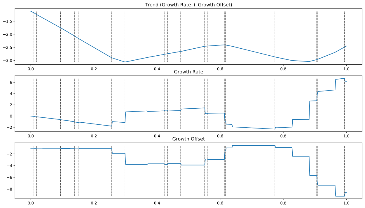
Explanations

Notice that where the defined \(N\) amount of changepoints (n_changepoints) resulted in the N-dimensional \(\delta\) tensor, dictating the “magnitudes” of our two terms, Growth Rate & Offsets, at those \(N\) specific changepoints in the numeric timesteps \(\boldsymbol{t}\), or simply at \(\boldsymbol{s}\). Together, they additively combined to produce the predicted “trend” of the observed.

Modeling Seasonal Components [\(\boldsymbol{S}_{m}(t)\) & \(\boldsymbol{S}_{a}(t)\)]

It is important to clarify that we actually are addressing more than one particular component (not \(m\) vs \(a\), though we will touch base on that soon). The seasonal components, by fbprophet’s point of view, although grouped as one, breaks down into 2 categories:

Seasonality: Cyclic nature of a given feature, such as a business operation exhibiting seasonal effects of sales due to certain periodic timeframe throughout the years, months or week. (e.g.: sales increase during summer & decrease during winter)
Holidays & Special Timeframes: Thanksgiving, New Year, Independence Day, Major Sport Events (SuperBowl, World Cup, etc), and many many more. These are somewhat seasonal & periodic, but they can also be a singular timeframe of a significant event in history (subjective to judgment), like COVID-19 & its impact on the financial market, or any special days we’d like to add that are relevant to the problem at hand.

Where

\(S_a =\) Additive Seasonal Components
\(S_m =\) Multiplicative Seasonal Components

Moving forward, we will primarily focus on the Seasonality aspect as Holidays & Special Timeframes are much easier to understand once we grasp trend & seasonality.

Seasonality & Fourier Series

In mathematics, the fourier series is an extremely powerful series that, shortly put, can represent any linear functions through regressing \(N\) (order) amount of factors of sine & cosine pairs, which are just combinations of drawing many circles under different initial conditions (aka where we place our pencils to start) then scale it to the center.

Cool Highlight: I highly recommend checking out this amazing clip, showing how fourier series can be used, through iterative regressions, to draw any given outlines.

To compute a fourier series as a seasonal effect throughout time, we simply set our independent variable as \(\boldsymbol{t}\), the scaled timestep, as that being the only information needed to make predictions. Although during the process of designing our model, we need to specify the series’ period & order for each seasonality component.

As each singular seasonality component being a fourier series with certain choice of period & order, we define it as \(F_{\lambda,N}(t)\), where:

\(\lambda\) = period (365.25 = annual, 7 = weekly, etc)
\(N\) = fourier order (amount of sine & consine pairs to add together to fit our objective)

Thus, we have:

\[F_{\lambda,N}(t) = \sum_{n=1}^{N}(a_{n} cos(\frac{2\pi nt}{\lambda}) + b_{n}sin(\frac{2\pi nt}{\lambda}))\]

where \(a_n\) and \(b_n\) are the pairs of coefficients for each term in the total of N pairs, whereas an order of \(N\) would resulted in \(2N\) coefficients for \(N\) components of wave-pairs. Using the advantage of matrices (like \(\delta\) dimension = the amount of changepoints in the trend model above), we seek to find the coefficients \(a_n\) and \(b_n\) as a \(2N\)-dimensional prior in our seasonality model with:

\[\boldsymbol{\beta} \sim \mathcal{N}(0,\phi)\]

where \(\phi\) is the scale hyperparameter, similar to \(\theta\) in our trend model above. While \(\theta = 5\) being recommended as default by fbprophet, \(\boldsymbol{\beta}\)’s scale \(\phi\) is defaulted as \(\phi = 10\). We define our prior \(\boldsymbol{\beta}\), with the default scale, as:

\[\boldsymbol{\beta} \sim \mathcal{N}(0,10)\] \[\boldsymbol{\beta} \in \mathbb{R}^{2N}, \boldsymbol{\beta} = a_1, b_1, …, a_n, b_n\]

As each seasonality component \(F_{\lambda,N}(t) \sim\) a fourier series with specified \(\lambda\) & \(N\), with the separated \(a_n,b_n\) with prior \(\boldsymbol{\beta}\), for any given \(t\), each component will have a transformed tensor from such \(t\), representing the sine & cosine terms, being

\[X(t) = [ cos(\frac{2\pi 1t}{\lambda}), sin(\frac{2\pi 1t}{\lambda}),…,cos(\frac{2\pi Nt}{\lambda}),sin(\frac{2\pi Nt}{\lambda}) ]\]

Thus, the seasonality component, in fourier series, \(F_{\lambda,N}(t)\), with the followed \(X(t)\), resulted in:

\[X(t) \boldsymbol{\beta} = \sum_{n=1}^{N}(a_{n} cos(\frac{2\pi nt}{\lambda}) + b_{n}sin(\frac{2\pi nt}{\lambda}))\]

or simply put, given a choice of \(\lambda,N\) resulted in \(X(t),\boldsymbol{\beta}\), we have:

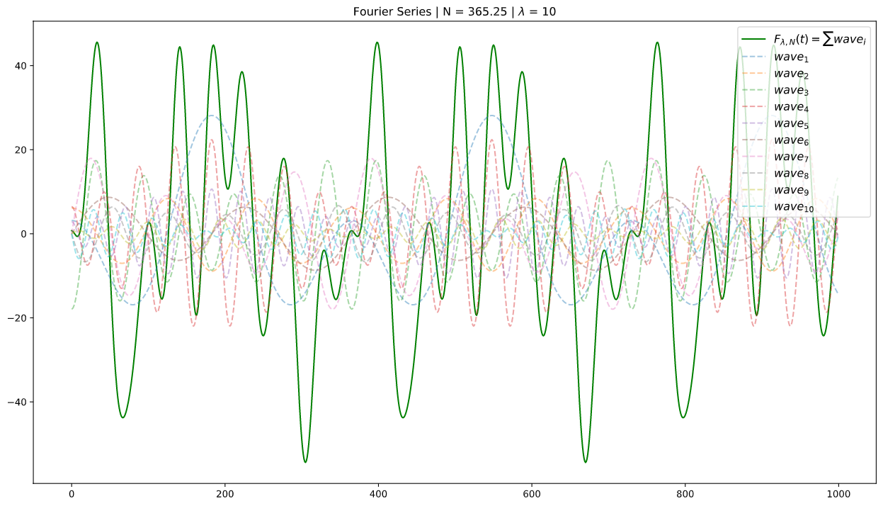
\[F_{\lambda,N}(t) = X(t) \boldsymbol{\beta}\]

Demonstrating Seasonality as Fourier Series

We first prepare a function that takes in \(\boldsymbol{t}\) as an array of scaled timesteps with length \(K\), along with the fourier properties \(\lambda\) (period) & \(N\) (order) as single values, to calculate the fourier series and return it as an array of dimension \(K\) x \(2N\):

def fourier_series(t, period, order):
    # 2 pi n / p
    x = 2 * np.pi * np.arange(1, order + 1) / period
    # 2 pi n / p * t
    x = x * t[:, None]
    x = np.concatenate((np.cos(x), np.sin(x)), axis=1)
    return x

With hyperparams set as fbprophet’s defaults for annual seasonality (at daily interval):

\[\lambda=365.25\]
\[N=10\]
\[\phi = 10\]

To obtain \(F_{\lambda,N}(t)\) as \(X(t) \boldsymbol{\beta}\), a single seasonality component with given numeric timestep(s) \(\boldsymbol{t}\), we demonstrate this by:

Randomly generate a sample of our \(2N\)-dimensional \(\beta\) prior defined with specified scale \(\phi\) (\(=10\) by default).
Perform fourier calculations using the fourier_series function written above to obtain \(X(t)\) with dimension \(K\) x \(2N\)

Performing matrix multiplication \(X(t) \boldsymbol{\beta}\) will resulted in a 1D array of length \(K\), or basically \(K\) x \(1\) as its matrix dimension, representing a singular sample (using generated \(\boldsymbol{\beta}\) sample) of the seasonality component \(s_i\) with given the choice of \(\lambda,N\), in our overarching seasonality model, either as multiplicative or additive (\(s_i \in S_m\) (or \(S_a\))).

In addition, I also include the \(N\) (order) wave components \(wave_i\) for \(i=1,2,...,N\), constructing our result in green, to show the additive contributions of any given order that allow for complexities for fitting by the fourier series.

t = np.arange(1000) #--| scaled timesteps in days for demonstration (1000 = 1000 date stamps per daily interval)
order = 10 #---| fourier order (N)
period = 365.25 #---| fourier period (lambda)
phi = 10 #---| beta's prior scale (a_n, b_n)

#----| Compute X & Beta
X = fourier_series(t,period,order)
beta = np.random.normal(0,phi,size=2 * order)

#----| Plot
plt.figure(figsize=(16, 9))
plt.subplot(111)
plt.title("Fourier Series | N = " + str(period) + " | $\lambda$ = " + str(order))
plt.plot(t,np.dot(X,beta), lw=1.5, color="green", label="$F_{\lambda,N}(t)=\sum wave_i$")

i = 0
for o in range(order):
    i +=1
    idx = o*2
    _latex = "$wave_{" + str(o + 1) + "}$"
    plt.plot(t,np.dot(X[:,idx:(idx+2)],beta[idx:(idx+2)]),"--",alpha=0.42, label = _latex)

plt.legend(loc="upper right",fontsize='large')
plt.autoscale(True)

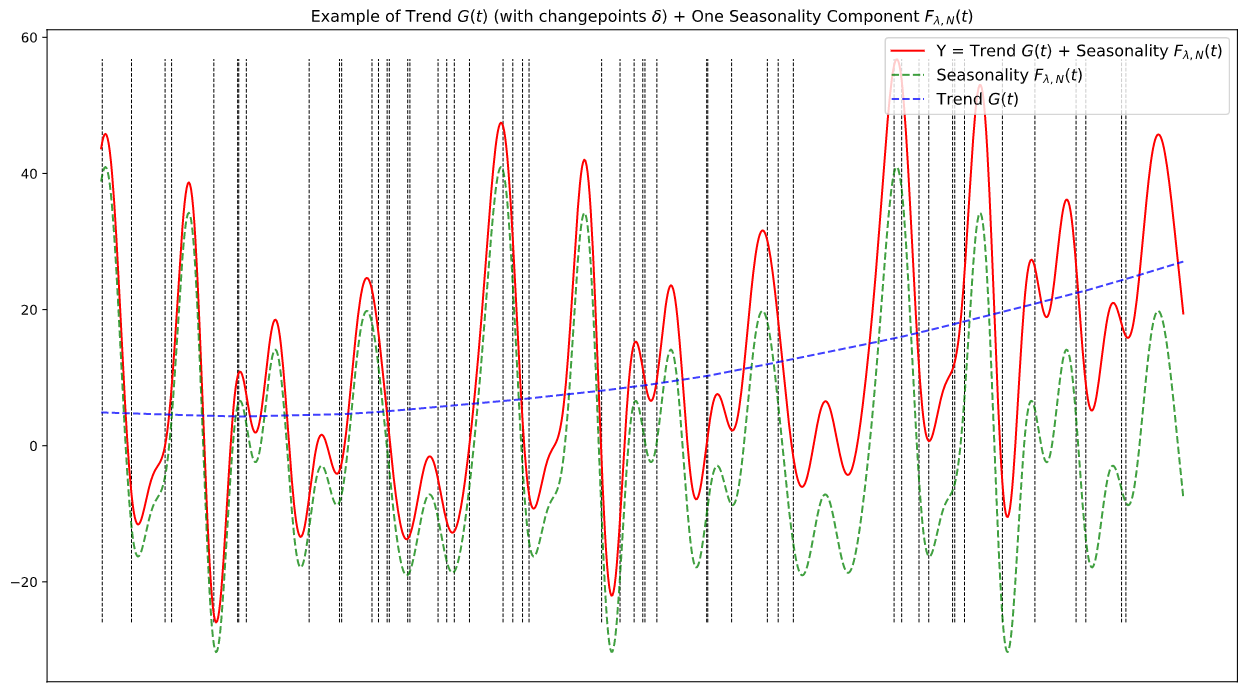
Visual Example of Combining Trend & Fourier Seasonality

As a quick recall of our overarching model being an additive linear of Trend & Seasonal Components, each is a model in itself, below is an example plot showing the two coming together to formulate the predicted Y.

Note that, again, this is just purely for demonstration where priors data are randomly generated, as there being no specific Y to fit our priors to:

Holidays & Special Timeframes

The difference compared to the Seasonlity model above simply resides in that instead of using the components of fourier series, \(F_{\lambda,N}\), that described above in \(X(t)\), we will instead use binaries to indicate when, or simply the timeframe(s), the holidays occur. We then proceed to perform multiplication with a regressed value in \(\boldsymbol{\beta}\) prior to obtain the Holidays & Special Timeframes component.

Using the example above, if we have our time-series data with timestamps \(D\) (for datetime), before we perform numerical transformation into \(t\), such that:

\[D = \begin{bmatrix} 1-2-2018 \\ 1-3-2018 \\ \vdots \\ 12-31-2018 \\ \vdots \\ 1-2-2020 \\ 1-3-2020 \end{bmatrix}\]

We construct the binary vector of the same length as \(D\), called \(H_{ny}\), such that we can model the New Year’s effect by defining the New Year’s timeframe starting from Dec-30 to Jan-2, thus assign those stamps with the value \(1\), and others as \(0\):

\[H_{ny} = \begin{bmatrix} 1 \\ 0 \\ \vdots \\ 1 \\ \vdots \\ 1 \\ 0 \end{bmatrix}\]

Regressively, after performing multiplication with a value in our \(\boldsymbol{\beta}\) prior, we obtain our New Year’s holiday effect, additive or multiplicative.

As I tried to keep this section as brief as possible due to its simplicity, if you want more information and examples, you can visit FBProphet’s documentation here.

Share on

Twitter Facebook Google+ LinkedIn

Jack Pham